Why people leave: what the stated reason hides
People Analytics
R
Quarto
Turnover
Two years of separations and exit interviews at a supermarket chain. Why people resign, where it concentrates and where to act first.
Fictional case. Cestária Supermercados, its stores, people and interviews do not exist. The data was generated from scratch by an R script, with patterns of known size. The method is real.
Download the report (PDF) · Download the priorities by department (CSV)
The question
Cestária is a supermarket chain in inland Minas Gerais, Brazil, with 8 stores (L1 to L8), a distribution center (DC) and a headquarters office (HQ), and about 1,790 people on staff. In 2024 and 2025, 1,453 people left the company.
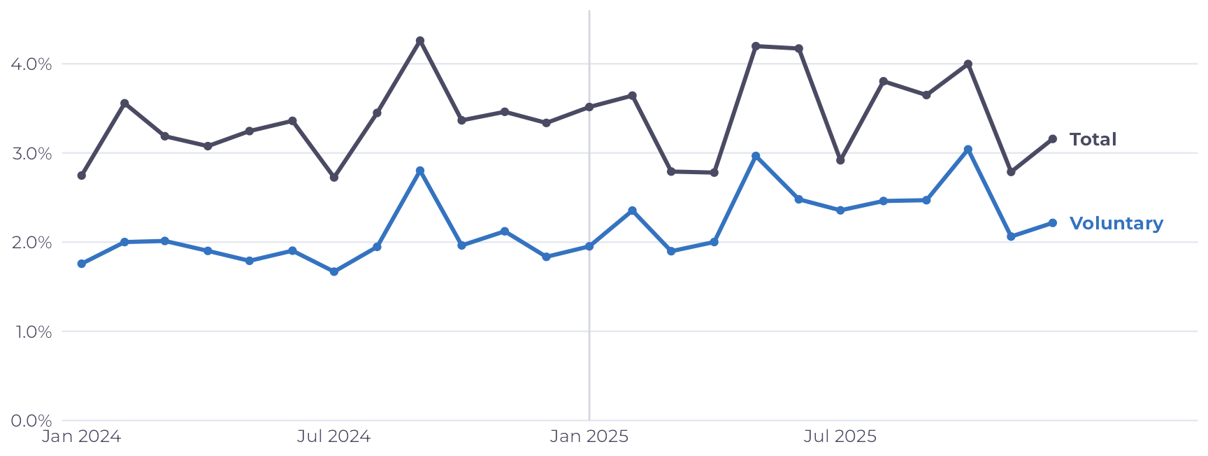
The separation rate did not move: on average, 3.31% of the workforce left each month in 2024 and 3.45% in 2025, a difference consistent with chance (p = .45). The mix, however, did change. Voluntary exits rose from 1.98% to 2.35% a month, and dismissals fell by almost the same amount.
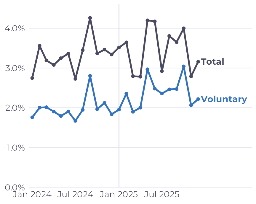
With a stable total, turnover did not look like an issue. Leadership asked two other questions instead: why do people resign, and where should we act first? To answer them, the exit interview, which the company already ran and nobody read alongside anything else, was crossed with the monthly headcount and the separations.
What the data shows
- The stated reason hides the real one. “Pay and benefits” is the reason most often given by people who resign (25.6%). Among those who rated their manager 1 or 2, however, “leadership and manager” moves ahead, at 44.5% against 20.9%.
- Exits in the first 90 days grew in two departments. In DC Shipping, the share of new hires who resigned within 90 days went from 20% in 2024 to 39% in 2025; in L3 Operations, from 20% to 41%. In the other departments, the figure stayed near 17%.
- L5 Sales started losing more people after its manager changed, in July 2025, and “leadership and manager” became the reason for 71% of the exits answered from then on.
- The 6x1 schedule on the night shift concentrates “hours and schedule”, the reason for 40% of exits in that group, against 8% everywhere else. The 6x1 schedule means six days on and one day off.
- Age does not explain the exits. Younger people leave more, but only because they have less tenure; with tenure in the model, the difference disappears.
- The interview has response bias, stronger for involuntary exits and at L7, but correcting for it does not change the order of the reasons.
What the stated reason hides
People who resign (resignation or mutual agreement) give, in the interview, a main reason and, optionally, a secondary one, from a closed list of eight. There were 712 responses with a reason over the two years.
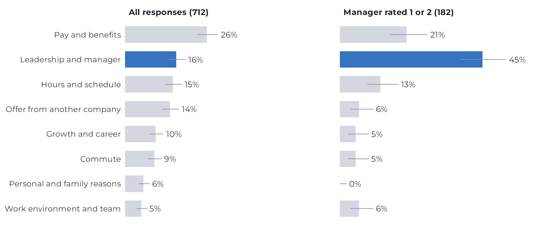
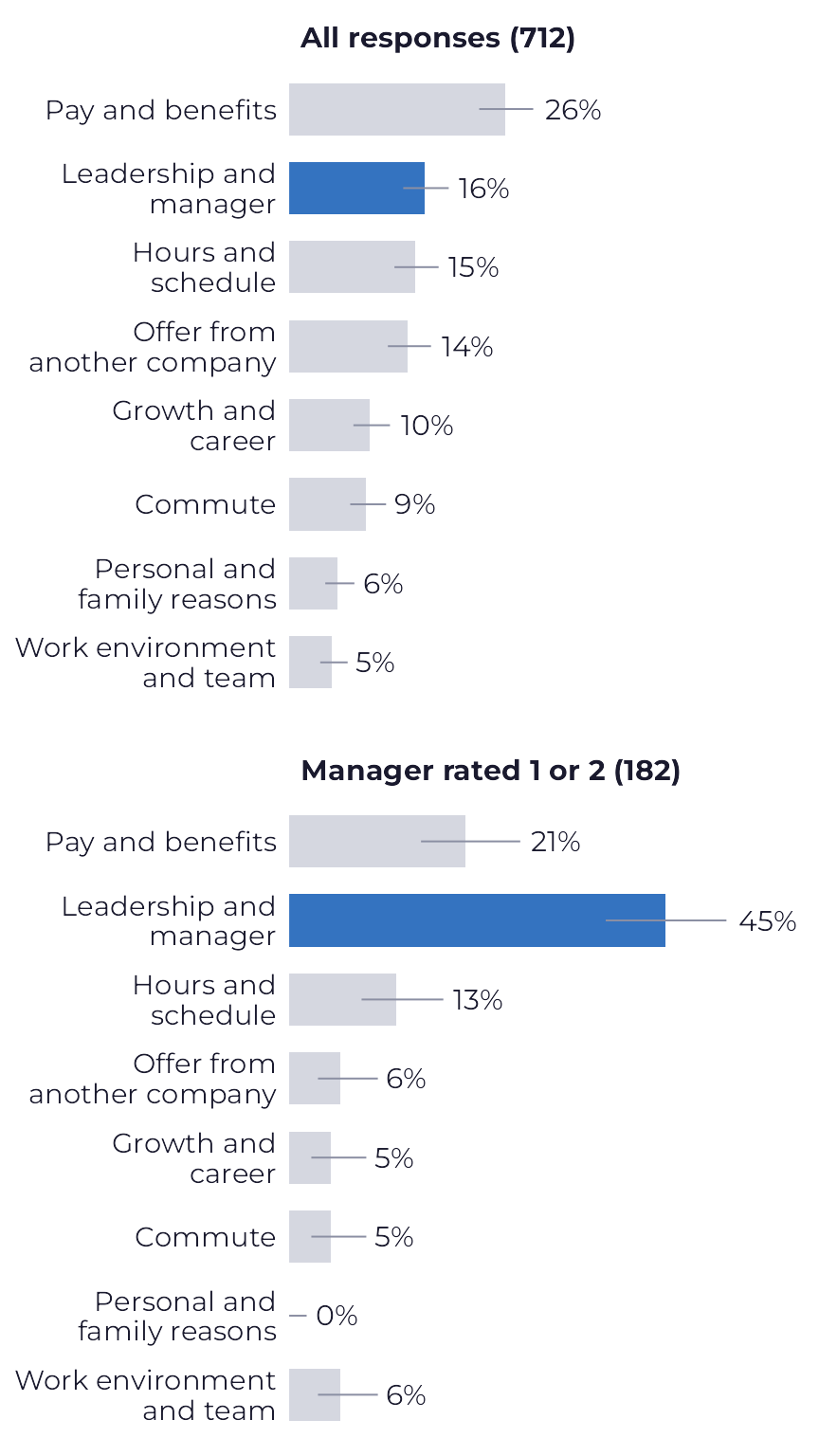
Overall, “pay and benefits” leads, with 25.6% of responses (95% CI 22.5% to 28.9%), and “leadership and manager” comes in at 16.0%. The picture changes among the 182 people who rated their manager 1 or 2: “leadership and manager” rises to 44.5% (37.5% to 51.8%), and pay drops to 20.9%.
Pay also hides leadership when it comes with a low rating. Of the 38 people who rated their manager 1 or 2 and gave pay as their main reason, 22 (58%) gave “leadership and manager” as their secondary reason. Counting main and secondary reasons together, 73% of those who rated their manager low mention leadership, against 15% of everyone else.
This does not prove that the manager caused the exit. It shows that the stated reason, read on its own, points to pay, while the manager rating and the secondary reason point to leadership. Pay is the easiest answer to give in an exit conversation; that is why the interview has to be read together with the rating and the second reason, not by the first reason alone.
Who answered the interview
The interview is not mandatory. Of those who resigned, 77% answered it, against only 38% of those who were dismissed. Among sites, L7 is well below the others, with a 37% response rate.
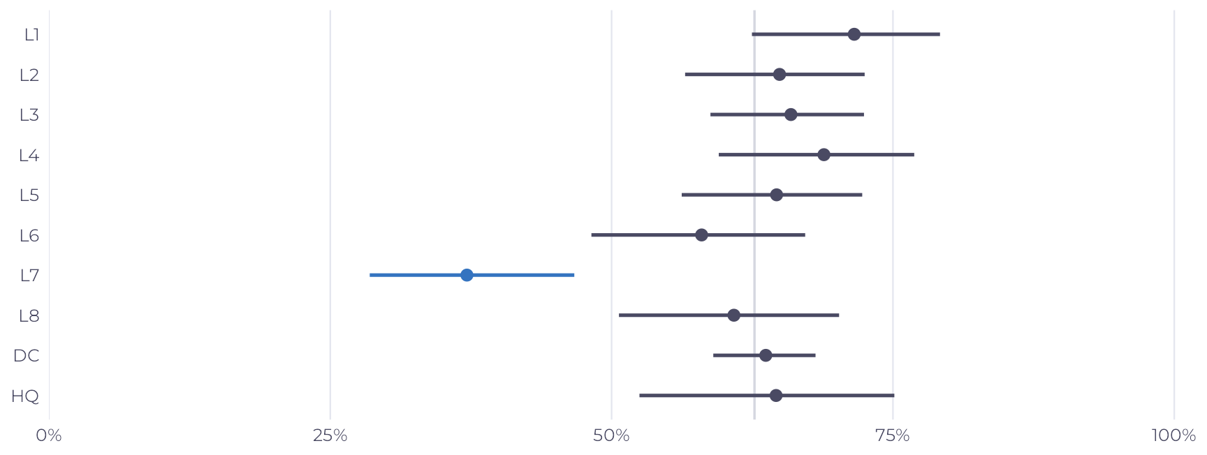
Because the reason is only asked of people who resign, the gap between voluntary and involuntary exits does not distort the picture of reasons; the gap between sites does. To see whether it changes the conclusion, each response was weighted by the inverse of its site’s response rate, so that L7 counts as much as it would if everyone had answered. No reason moved by more than 0.3 percentage point, and the order stayed the same.
| Reason | Unweighted | Weighted |
|---|---|---|
| Pay and benefits | 25.6% | 25.6% |
| Leadership and manager | 16.0% | 15.9% |
| Hours and schedule | 14.9% | 14.9% |
| Offer from another company | 14.0% | 14.0% |
| Growth and career | 9.6% | 9.4% |
| Commute | 9.1% | 8.9% |
| Personal and family reasons | 5.8% | 6.0% |
| Work environment and team | 5.1% | 5.2% |
Pay and benefits
Unweighted: 25.6%
Weighted: 25.6%
Leadership and manager
Unweighted: 16.0%
Weighted: 15.9%
Hours and schedule
Unweighted: 14.9%
Weighted: 14.9%
Offer from another company
Unweighted: 14.0%
Weighted: 14.0%
Growth and career
Unweighted: 9.6%
Weighted: 9.4%
Commute
Unweighted: 9.1%
Weighted: 8.9%
Personal and family reasons
Unweighted: 5.8%
Weighted: 6.0%
Work environment and team
Unweighted: 5.1%
Weighted: 5.2%
The weighting assumes that, within each site, the people who answered are similar to those who did not. If those who did not answer at L7 left for different reasons than those who did, no weight can fix that; it is the first of the case’s limitations.
Where to act first
Exits in the first 90 days
Among the 1,222 people hired from January 2024 to October 2, 2025, who have already reached 90 days of tenure, the share who resigned by day 90 rose in two departments and held steady everywhere else. In DC Shipping, it went from 20% among 2024 hires to 39% among 2025 hires (95% CI 31% to 48%); in L3 Operations, from 20% to 41% (26% to 57%). In the other departments, from 15% to 17%.
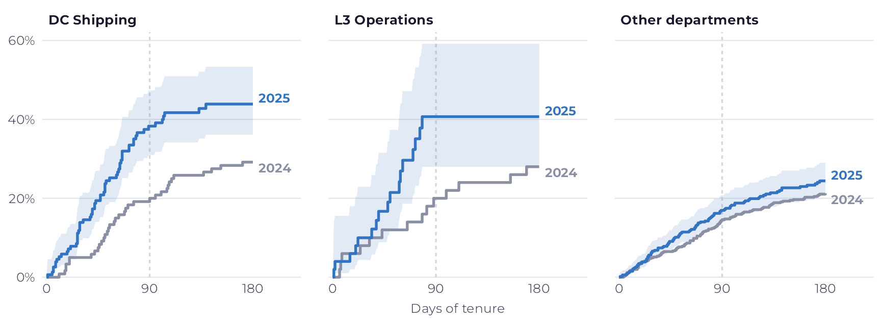
In a cause-specific Cox model with 2025 hires only, the risk of voluntary exit was 2.2 times that of the other departments in DC Shipping (95% CI 1.6 to 3.0) and 2.1 times in L3 Operations (1.3 to 3.5).
Leaving in the first 90 days usually has more to do with onboarding than with the job market: the induction, the schedule described at hiring, the first manager. Neither department changed managers, and the interview of someone who leaves that early is short; the next step is to listen to new hires in those two areas before they reach 90 days.
The manager change in L5 Sales
L5 Sales changed managers in July 2025. To separate the effect of the change from what happened across the company in the same period, L5 was compared with the other seven Sales departments, which kept their managers.
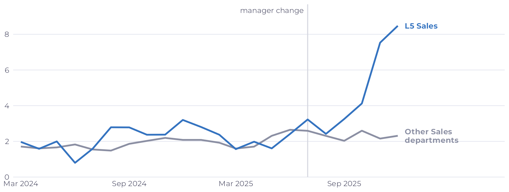
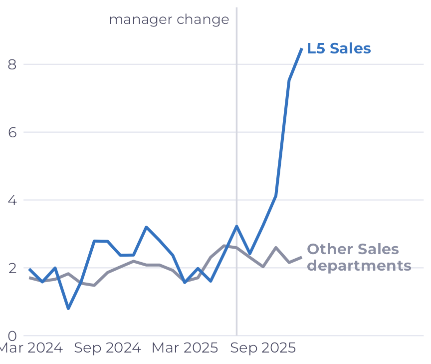
Before the change, L5 lost 2.1% of its staff a month to voluntary exits, and the other Sales departments, 2.0%. Afterward, L5 went to 5.8%, and the others, to 2.2%. Netting out the change in the other departments, the L5 rate was 2.5 times higher after the manager change (95% CI 1.4 to 4.4, Poisson model).
The reason follows: before the change, “leadership and manager” came up in fewer than 10 of the 25 L5 responses; afterward, in 17 of 24 (71%, 51% to 85%). It is an association in time, not proof that the new manager is the cause: there are only six months of data, and something else may have changed at the store at the same time. But it is the strongest signal in the case, and the cheapest to check, in a conversation with the team and with the manager.
The 6x1 schedule on the night shift
On the 6x1 night shift, which covers restocking at the stores and part of the DC, “hours and schedule” is the reason for 40% of the voluntary exits answered (33% to 48%), against 8% in the other shift and schedule combinations. The voluntary exit rate is also the highest: 2.80% of the group a month.
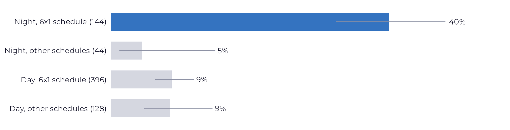
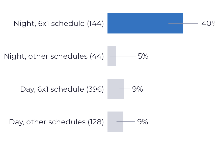
Night work on other schedules (12x36 at the DC, 5x2 at some stores) does not have the same problem. What weighs is the combination of night work with a single day off a week, and that points to a scheduling decision, not a pay decision.
Priorities by department
The three fronts above become a list. For 2025, each department received a priority:
- High: the voluntary exit rate or the share of new hires who left within 90 days is above the company even at the lower bound of the confidence interval.
- Medium: both are above the company in the point estimate, or “leadership and manager” or “hours and schedule” are above the company at the lower bound of the interval.
- Monitor: everything else.
Within each level, the order follows voluntary exits above what the company rate would predict. The full list, with the intervals, is in the CSV at the top of the page; no figure for a group of fewer than 10 people appears in it.
L2 Operations stands out for “hours and schedule” in the reason by department cross-tab, but stays at “Monitor”: in 2025, its voluntary rate (2.82% a month) is above the company (2.35%) only in the point estimate, its exits within 90 days (6%) are below the company (24%), and the share of “hours and schedule” among its 2025 responses does not exceed the company at the lower bound of the interval.
| Rank | Department | Priority | Signals | Monthly voluntary rate | Exits within 90 days | Response | Leadership and manager |
|---|---|---|---|---|---|---|---|
| 1 | DC Shipping | High | Voluntary rate; Exits within 90 days | 3.21% | 39% | 63% | 16% |
| 2 | L5 Sales | High | Voluntary rate; Leadership and manager | 3.85% | 25% | 76% | 55% |
| 3 | L3 Operations | High | Exits within 90 days | 2.84% | 41% | 57% | 8% |
| 4 | L1 Operations | Medium | Voluntary rate (point estimate); Exits within 90 days (point estimate) | 3.60% | 30% | 77% | 6% |
| 5 | L2 Operations | Monitor | Hours and schedule (reason by department) | 2.82% | 6% | 64% | 23% |
| 6 | L3 Sales | Monitor | 2.50% | 19% | 68% | 21% | |
| 7 | L8 Sales | Monitor | 2.42% | 20% | 74% | 26% | |
| 8 | L6 Operations | Monitor | 2.28% | 24% | 78% | 31% | |
| 9 | L5 Operations | Monitor | 2.18% | 21% | 54% | <10 | |
| 10 | L4 Sales | Monitor | 2.20% | 29% | 71% | 21% | |
| 11 | L8 Operations | Monitor | 1.99% | 12% | 60% | <10 | |
| 12 | L1 Sales | Monitor | 2.11% | 17% | 65% | 27% | |
| 13 | L6 Sales | Monitor | 2.11% | 19% | 53% | 7% | |
| 14 | L7 Operations | Monitor | 1.97% | 21% | 22% | <10 | |
| 15 | L4 Operations | Monitor | 1.85% | 7% | 84% | 0% | |
| 16 | L2 Sales | Monitor | 2.02% | 13% | 69% | 11% | |
| 17 | L7 Sales | Monitor | 1.58% | 6% | 32% | <10 | |
| 18 | DC Receiving | Monitor | 2.01% | 18% | 62% | 8% | |
| 19 | HQ Administration | Monitor | 0.94% | 4% | 72% | 15% |
1. DC Shipping
Priority: High
Signals: Voluntary rate; Exits within 90 days
Monthly voluntary rate: 3.21%
Exits within 90 days: 39%
Response: 63%
Leadership and manager: 16%
2. L5 Sales
Priority: High
Signals: Voluntary rate; Leadership and manager
Monthly voluntary rate: 3.85%
Exits within 90 days: 25%
Response: 76%
Leadership and manager: 55%
3. L3 Operations
Priority: High
Signals: Exits within 90 days
Monthly voluntary rate: 2.84%
Exits within 90 days: 41%
Response: 57%
Leadership and manager: 8%
4. L1 Operations
Priority: Medium
Signals: Voluntary rate (point estimate); Exits within 90 days (point estimate)
Monthly voluntary rate: 3.60%
Exits within 90 days: 30%
Response: 77%
Leadership and manager: 6%
5. L2 Operations
Priority: Monitor
Signals: Hours and schedule (reason by department)
Monthly voluntary rate: 2.82%
Exits within 90 days: 6%
Response: 64%
Leadership and manager: 23%
6. L3 Sales
Priority: Monitor
Monthly voluntary rate: 2.50%
Exits within 90 days: 19%
Response: 68%
Leadership and manager: 21%
7. L8 Sales
Priority: Monitor
Monthly voluntary rate: 2.42%
Exits within 90 days: 20%
Response: 74%
Leadership and manager: 26%
8. L6 Operations
Priority: Monitor
Monthly voluntary rate: 2.28%
Exits within 90 days: 24%
Response: 78%
Leadership and manager: 31%
9. L5 Operations
Priority: Monitor
Monthly voluntary rate: 2.18%
Exits within 90 days: 21%
Response: 54%
Leadership and manager: <10
10. L4 Sales
Priority: Monitor
Monthly voluntary rate: 2.20%
Exits within 90 days: 29%
Response: 71%
Leadership and manager: 21%
11. L8 Operations
Priority: Monitor
Monthly voluntary rate: 1.99%
Exits within 90 days: 12%
Response: 60%
Leadership and manager: <10
12. L1 Sales
Priority: Monitor
Monthly voluntary rate: 2.11%
Exits within 90 days: 17%
Response: 65%
Leadership and manager: 27%
13. L6 Sales
Priority: Monitor
Monthly voluntary rate: 2.11%
Exits within 90 days: 19%
Response: 53%
Leadership and manager: 7%
14. L7 Operations
Priority: Monitor
Monthly voluntary rate: 1.97%
Exits within 90 days: 21%
Response: 22%
Leadership and manager: <10
15. L4 Operations
Priority: Monitor
Monthly voluntary rate: 1.85%
Exits within 90 days: 7%
Response: 84%
Leadership and manager: 0%
16. L2 Sales
Priority: Monitor
Monthly voluntary rate: 2.02%
Exits within 90 days: 13%
Response: 69%
Leadership and manager: 11%
17. L7 Sales
Priority: Monitor
Monthly voluntary rate: 1.58%
Exits within 90 days: 6%
Response: 32%
Leadership and manager: <10
18. DC Receiving
Priority: Monitor
Monthly voluntary rate: 2.01%
Exits within 90 days: 18%
Response: 62%
Leadership and manager: 8%
19. HQ Administration
Priority: Monitor
Monthly voluntary rate: 0.94%
Exits within 90 days: 4%
Response: 72%
Leadership and manager: 15%
What does not explain it: age
Looking at age alone, younger people leave more: the odds of someone aged 18 to 24 resigning in a given month are 1.60 times those of someone aged 35 to 44 (95% CI 1.33 to 1.94). But younger people have, on average, the least tenure, and tenure is what matters: with it in the model, the ratio drops to 1.01 (0.83 to 1.24), and age group as a whole stops making a difference (p = .40).
It is a null finding that matters: a policy “to retain young people” would aim at the wrong target. The point of attention is the first months on the job, at any age.
Limitations
- Fictional data. The patterns were planted by a generator, and the analysis found them without reading the answer key. With real data, the figures would differ; the method is the same.
- Response bias. The weighting corrects the difference in response between sites, but assumes that, within each site, the people who answered are similar to those who did not. That cannot be checked with this data.
- Association is not causation. The comparison of L5 with the other Sales departments assumes that, without the change, L5 would have followed the same trend as they did. With six months after the change, the interval is still wide.
- Stated reason. The list is closed, and each person picks one main reason; it is what they say, not necessarily what weighed most.
- 90-day window. People hired after October 2, 2025 are left out of that count, because they have not yet completed the window.
- Many comparisons. In the reason by department cross-tab, only adjusted residuals with an absolute value of 3 or more count as standouts.
Method
The steps are in the code, each one in a collapsed block; the technical tables are at the end of the section.
- Classify exits. Voluntary means resignation; involuntary means dismissal without cause and end of probation. Mutual agreement is its own category and counts as voluntary in the two-way split (930 voluntary and 523 involuntary over the two years).
- Separation rate. Separations in the month ÷ average headcount for the month, where average headcount is the mean of the headcount on the first and last day. The classic turnover formula uses the average of hires and separations as the numerator. Over a year, the two give almost the same result: the separation rate was 39.8% in 2024 and 41.4% in 2025, and classic turnover, 38.8% and 41.3%. Rate intervals are exact Poisson intervals, per person-month.
- Exits within 90 days. Among people hired from January 2024 to October 2, 2025 (1,222), those who resigned by day 90 of tenure. Anyone dismissed before 90 days counts as “did not resign”.
- Reasons. Pareto of the main reason among people who resigned and answered, overall and with a manager rating of 1 or 2; proportions with Wilson intervals.
- Response rate and weighting. Response rate by exit type and by site, and the Pareto weighted by the inverse of the site’s response rate.
- Reason by department. Chi-square test of independence (115.1 with 90 degrees of freedom), with the three least cited reasons combined into “other reasons” and the p-value computed by simulation (p = .035), because 56% of the cells have an expected frequency below 5. Standouts only for adjusted residuals with an absolute value of 3 or more: L5 Sales in “leadership and manager” (4.9) and L2 Operations in “hours and schedule” (3.0).
- Cumulative incidence and cause-specific Cox. Time from hiring day to exit, for people hired in 2024 and 2025, with involuntary exit as a competing risk (Aalen-Johansen estimator,
survfitfrom the survival package with the status as a factor). In place of Gray’s test, which needs a package that is not installed, a cause-specific Cox model: department as a whole is associated with the risk of voluntary exit (likelihood ratio test, 62.5 with 18 degrees of freedom, p < .001). - Manager change. Voluntary exits by Sales department and month, with exposure in person-months, in a Poisson model with department, period (before or after July 2025) and the interaction of L5 with the post-change period (difference in differences). The negative binomial model would be used if dispersion exceeded 1.2; it was 0.96.
- Logistic regression. Resignation within 90 days, with the department group, hiring year and their interaction, the night 6x1 schedule and age group.
- Confounding by age. Person-month logistic regression of resignation in the month, with age group alone and then with tenure band.
- Priorities. The criteria from the previous section, applied to 2025, with figures for groups of fewer than 10 people replaced by “<10”.
Show the R code: separation rate
# Taxa de desligamento do mês: desligamentos ÷ headcount médio, em que o
# headcount médio é a média entre o quadro do primeiro e do último dia.
# A fórmula clássica de turnover usa a média entre admissões e desligamentos
# no numerador; as duas aparecem no método.
mensal <- pessoa_mes |>
  group_by(ano_mes) |>
  summarise(hc_medio = sum(peso), admissoes = sum(admitido_no_mes), .groups = "drop") |>
  left_join(saidas |> count(ano_mes, name = "desligamentos"), "ano_mes") |>
  left_join(saidas |> filter(voluntaria) |> count(ano_mes, name = "voluntarios"), "ano_mes") |>
  mutate(across(c(desligamentos, voluntarios), \(x) coalesce(x, 0L)),
         taxa = 100 * desligamentos / hc_medio, taxa_vol = 100 * voluntarios / hc_medio,
         turnover_classico = 100 * (admissoes + desligamentos) / 2 / hc_medio)

anual <- mensal |>
  group_by(ano = as.integer(substr(ano_mes, 1, 4))) |>
  summarise(exposicao = sum(hc_medio), hc_medio = exposicao / n(), desligamentos = sum(desligamentos),
            voluntarios = sum(voluntarios), involuntarios = desligamentos - voluntarios,
            admissoes = sum(admissoes), .groups = "drop") |>
  # Taxa mensal média (por pessoa-mês) e taxa do ano (desligamentos do ano ÷
  # headcount médio do ano).
  mutate(taxa_ano = 100 * desligamentos / hc_medio, taxa_vol_ano = 100 * voluntarios / hc_medio,
         taxa = 100 * desligamentos / exposicao,
         taxa_inf = taxa_ic(desligamentos, exposicao, "inf"), taxa_sup = taxa_ic(desligamentos, exposicao, "sup"),
         taxa_vol = 100 * voluntarios / exposicao,
         taxa_vol_inf = taxa_ic(voluntarios, exposicao, "inf"), taxa_vol_sup = taxa_ic(voluntarios, exposicao, "sup"),
         taxa_inv = 100 * involuntarios / exposicao,
         turnover_classico = 100 * (admissoes + desligamentos) / 2 / exposicao,
         turnover_classico_ano = 100 * (admissoes + desligamentos) / 2 / hc_medio)
teste_anos <- poisson.test(anual$desligamentos, anual$exposicao)

tipos <- saidas |> count(tipo) |> mutate(pct = 100 * n / sum(n))
Show the R code: exits within 90 days
# Saídas voluntárias até 90 dias, entre os admitidos no período. Ficam fora os
# admitidos depois de 02/10/2025, que ainda não completaram a janela. Quem foi
# dispensado antes dos 90 dias conta como "não saiu voluntariamente".
coorte <- colaborador |>
  filter(data_admissao >= as.Date("2024-01-01")) |>
  left_join(pessoa_mes |> distinct(id_colaborador, gerencia, unidade) |> distinct(id_colaborador, .keep_all = TRUE),
            "id_colaborador") |>
  left_join(deslig |> select(id_colaborador, data_desligamento, tipo), "id_colaborador") |>
  mutate(ano_admissao = year(data_admissao),
         dias = as.integer(coalesce(data_desligamento, FIM) - data_admissao),
         vol_90 = !is.na(tipo) & tipo %in% VOLUNTARIOS & dias <= 90,
         noite_6x1 = turno == "Noite" & escala == "6x1",
         grupo = if_else(gerencia %in% c("L3 Operações", "CD Expedição"), gerencia, "Demais gerências"))
coorte_90 <- coorte |> filter(data_admissao <= JANELA_90)

noventa_ano <- coorte_90 |>
  group_by(ano_admissao) |>
  summarise(admitidos = n(), saidas = sum(vol_90), .groups = "drop") |>
  mutate(pct = 100 * saidas / admitidos, inf = wilson(saidas, admitidos, "inf"), sup = wilson(saidas, admitidos, "sup"))
noventa_gerencia <- coorte_90 |>
  group_by(gerencia, ano_admissao) |>
  summarise(admitidos = n(), saidas = sum(vol_90), .groups = "drop") |>
  mutate(pct = 100 * saidas / admitidos, inf = wilson(saidas, admitidos, "inf"), sup = wilson(saidas, admitidos, "sup"),
         gerencia = factor(gerencia, ordem_gerencias))
# Diferença 2025 menos 2024 em cada gerência: as duas que mais sobem.
subida_90 <- noventa_gerencia |>
  select(gerencia, ano_admissao, pct, admitidos) |>
  pivot_wider(names_from = ano_admissao, values_from = c(pct, admitidos)) |>
  mutate(diferenca = pct_2025 - pct_2024) |>
  arrange(desc(diferenca))
noventa_grupo <- coorte_90 |>
  group_by(grupo, ano_admissao) |>
  summarise(admitidos = n(), saidas = sum(vol_90), .groups = "drop") |>
  mutate(pct = 100 * saidas / admitidos, inf = wilson(saidas, admitidos, "inf"), sup = wilson(saidas, admitidos, "sup"))
Show the R code: reasons
# Motivo declarado: só quem pediu para sair (pedido ou acordo) e respondeu.
# Pareto geral e entre quem deu nota 1 ou 2 ao gestor.
respondentes <- saidas |> filter(voluntaria, respondeu == "Sim", !is.na(motivo_principal))
pareto <- function(d) {
  d |>
    count(motivo = motivo_principal) |>
    complete(motivo = MOTIVOS, fill = list(n = 0)) |>
    mutate(total = sum(n), pct = 100 * n / total, inf = wilson(n, total, "inf"), sup = wilson(n, total, "sup")) |>
    arrange(desc(n))
}
pareto_geral <- pareto(respondentes)
nota_baixa <- respondentes |> filter(nota_gestor <= 2)
pareto_nota_baixa <- pareto(nota_baixa)
# Quem declarou salário e deu nota baixa ao gestor: quantos põem a liderança
# como motivo secundário.
salario_nota_baixa <- nota_baixa |>
  filter(motivo_principal == "Salário e benefícios") |>
  summarise(n = n(), lideranca_secundario = sum(motivo_secundario %in% "Liderança e gestor")) |>
  mutate(pct = 100 * lideranca_secundario / n, inf = wilson(lideranca_secundario, n, "inf"),
         sup = wilson(lideranca_secundario, n, "sup"))
# Liderança citada como motivo principal ou secundário.
lideranca_qualquer <- respondentes |>
  mutate(nota_baixa = nota_gestor <= 2,
         lideranca = motivo_principal == "Liderança e gestor" | motivo_secundario %in% "Liderança e gestor") |>
  group_by(nota_baixa) |>
  summarise(n = n(), x = sum(lideranca), .groups = "drop") |>
  mutate(pct = 100 * x / n, inf = wilson(x, n, "inf"), sup = wilson(x, n, "sup"))
Show the R code: response rate and weighting
# Taxa de resposta da entrevista e ponderação pela inversa da taxa de resposta.
resposta_tipo <- saidas |>
  group_by(voluntaria) |>
  summarise(saidas = n(), responderam = sum(respondeu == "Sim"), .groups = "drop") |>
  mutate(pct = 100 * responderam / saidas, inf = wilson(responderam, saidas, "inf"),
         sup = wilson(responderam, saidas, "sup"))
resposta_unidade <- saidas |>
  group_by(unidade) |>
  summarise(saidas = n(), responderam = sum(respondeu == "Sim"), .groups = "drop") |>
  mutate(pct = 100 * responderam / saidas, inf = wilson(responderam, saidas, "inf"),
         sup = wilson(responderam, saidas, "sup"),
         unidade = factor(unidade, unique(estrutura$unidade)))
# Peso de cada resposta voluntária: saídas voluntárias da unidade ÷ respostas
# voluntárias da unidade. Supõe que, dentro de cada unidade, quem respondeu é
# parecido com quem não respondeu.
pesos <- saidas |>
  filter(voluntaria) |>
  group_by(unidade) |>
  summarise(peso = n() / sum(respondeu == "Sim" & !is.na(motivo_principal)), .groups = "drop")
pareto_ponderado <- respondentes |>
  left_join(pesos, "unidade") |>
  group_by(motivo = motivo_principal) |>
  summarise(peso = sum(peso), .groups = "drop") |>
  mutate(pct = 100 * peso / sum(peso)) |>
  right_join(pareto_geral |> select(motivo, pct_sem_peso = pct), "motivo") |>
  mutate(pct = coalesce(pct, 0), diferenca = pct - pct_sem_peso) |>
  arrange(desc(pct))
Show the R code: reason by department
# Motivo × gerência: qui-quadrado com p por simulação (mesmo agrupando, há
# células com frequência esperada pequena) e resíduos ajustados. Os três
# motivos menos citados viram "Outros motivos". Só |resíduo| >= 3 é destaque,
# por causa das muitas comparações.
MOTIVOS_QUI <- c(MOTIVOS[1:4], "Crescimento e carreira", "Outros motivos")
motivo_qui <- if_else(respondentes$motivo_principal %in% MOTIVOS_QUI, respondentes$motivo_principal, "Outros motivos")
tabela_mg <- table(factor(respondentes$gerencia, ordem_gerencias), factor(motivo_qui, MOTIVOS_QUI))
qui <- suppressWarnings(chisq.test(tabela_mg, simulate.p.value = TRUE, B = 20000))
qui_assint <- suppressWarnings(chisq.test(tabela_mg))
residuos <- as_tibble(as.table(qui$stdres), .name_repair = ~ c("gerencia", "motivo", "residuo")) |>
  left_join(as_tibble(tabela_mg, .name_repair = ~ c("gerencia", "motivo", "n")), c("gerencia", "motivo")) |>
  mutate(destaque = abs(residuo) >= 3)
Show the R code: cumulative incidence and Cox
# Incidência acumulada da saída voluntária com a involuntária como risco
# competitivo (Aalen-Johansen), entre os admitidos no período, até 180 dias.
coorte_ce <- coorte |>
  mutate(evento = factor(case_when(is.na(tipo) ~ "censura", tipo %in% VOLUNTARIOS ~ "voluntária",
                                   TRUE ~ "involuntária"), c("censura", "voluntária", "involuntária")),
         dias = pmax(dias, 0.5))
aj <- survfit(Surv(dias, evento) ~ grupo + ano_admissao, data = coorte_ce)
incidencia <- {
  s <- summary(aj, times = 0:180, extend = TRUE)
  col <- which(s$states == "voluntária")
  tibble(estrato = as.character(s$strata), dias = s$time, inc = 100 * s$pstate[, col],
         inf = 100 * s$lower[, col], sup = 100 * s$upper[, col]) |>
    mutate(grupo = str_match(estrato, "grupo=([^,]+)")[, 2],
           ano_admissao = as.integer(str_match(estrato, "ano_admissao=(\\d+)")[, 2]))
}
incidencia_90 <- incidencia |> filter(dias == 90)
# Cox causa-específico (a saída involuntária vira censura): teste global da
# gerência, no lugar do log-rank, e razão de riscos dos dois grupos em 2025.
cox_global <- coxph(Surv(dias, evento == "voluntária") ~ gerencia, data = coorte_ce)
teste_gerencia <- anova(cox_global)
cox_2025 <- coxph(Surv(dias, evento == "voluntária") ~ relevel(factor(grupo), "Demais gerências"),
                  data = filter(coorte_ce, ano_admissao == 2025))
hr_2025 <- broom::tidy(cox_2025, exponentiate = TRUE, conf.int = TRUE) |>
  mutate(grupo = sub(".*\\)", "", term)) |>
  select(grupo, hr = estimate, inf = conf.low, sup = conf.high, p = p.value)
Show the R code: manager change
# L5 Vendas troca de gestor em julho de 2025. Comparação de antes e depois com
# as outras sete gerências de Vendas como controle: saídas voluntárias por
# pessoa-mês, com modelo binomial negativo (diferença em diferenças).
vendas <- pessoa_mes |>
  filter(area == "Vendas") |>
  group_by(gerencia, ano_mes) |>
  summarise(hc = sum(peso), .groups = "drop") |>
  left_join(saidas |> filter(voluntaria, area == "Vendas") |> count(gerencia, ano_mes, name = "vol"),
            c("gerencia", "ano_mes")) |>
  mutate(vol = coalesce(vol, 0L), depois = as.Date(paste0(ano_mes, "-01")) >= TROCA,
         troca = gerencia == gerencia_troca, troca_depois = troca & depois)
# Poisson primeiro; se a dispersão passar de 1,2, binomial negativo.
formula_troca <- vol ~ gerencia + depois + troca_depois + offset(log(hc))
modelo_troca <- glm(formula_troca, family = poisson, data = vendas)
dispersao <- sum(residuals(modelo_troca, type = "pearson")^2) / df.residual(modelo_troca)
if (dispersao > 1.2) modelo_troca <- MASS::glm.nb(formula_troca, data = vendas)
rr_troca <- {
  b <- coef(summary(modelo_troca))["troca_depoisTRUE", ]
  tibble(rr = exp(b[["Estimate"]]), inf = exp(b[["Estimate"]] - 1.96 * b[["Std. Error"]]),
         sup = exp(b[["Estimate"]] + 1.96 * b[["Std. Error"]]), p = b[[4]], dispersao = dispersao,
         modelo = if (dispersao > 1.2) "binomial negativo" else "Poisson")
}
troca_taxas <- vendas |>
  group_by(grupo = if_else(troca, gerencia_troca, "Outras gerências de Vendas"), depois) |>
  summarise(vol = sum(vol), exposicao = sum(hc), .groups = "drop") |>
  mutate(taxa = 100 * vol / exposicao, inf = taxa_ic(vol, exposicao, "inf"), sup = taxa_ic(vol, exposicao, "sup"))
troca_mensal <- vendas |>
  group_by(grupo = if_else(troca, gerencia_troca, "Outras gerências de Vendas"), ano_mes) |>
  summarise(vol = sum(vol), hc = sum(hc), .groups = "drop") |>
  arrange(grupo, ano_mes) |>
  group_by(grupo) |>
  # Média móvel de três meses: a taxa de uma gerência só oscila muito mês a mês.
  mutate(taxa_mm3 = 100 * zoo_soma(vol) / zoo_soma(hc)) |>
  ungroup()
troca_lideranca <- respondentes |>
  filter(gerencia == gerencia_troca) |>
  group_by(depois = data_desligamento >= TROCA) |>
  summarise(n = n(), x = sum(motivo_principal == "Liderança e gestor"), .groups = "drop") |>
  mutate(pct = 100 * x / n, inf = wilson(x, n, "inf"), sup = wilson(x, n, "sup"))
Show the R code: schedule and shift
# Escala 6x1 no turno da noite: participação de "jornada e escala" entre os
# motivos e taxa de saída voluntária, contra as outras combinações.
grupo_jornada <- function(turno, escala) {
  case_when(turno == "Noite" & escala == "6x1" ~ "Noite, 6x1", turno == "Noite" ~ "Noite, outras escalas",
            escala == "6x1" ~ "Dia, 6x1", TRUE ~ "Dia, outras escalas")
}
ordem_jornada <- c("Noite, 6x1", "Noite, outras escalas", "Dia, 6x1", "Dia, outras escalas")
jornada <- respondentes |>
  group_by(grupo = factor(grupo_jornada(turno, escala), ordem_jornada)) |>
  summarise(n = n(), x = sum(motivo_principal == "Jornada e escala"), .groups = "drop") |>
  mutate(pct = 100 * x / n, inf = wilson(x, n, "inf"), sup = wilson(x, n, "sup")) |>
  left_join(pessoa_mes |>
              group_by(grupo = factor(grupo_jornada(turno, escala), ordem_jornada)) |>
              summarise(exposicao = sum(peso), pessoas = n_distinct(id_colaborador), .groups = "drop") |>
              left_join(saidas |> filter(voluntaria) |>
                          count(grupo = factor(grupo_jornada(turno, escala), ordem_jornada), name = "vol"), "grupo") |>
              mutate(taxa_vol = 100 * vol / exposicao, taxa_inf = taxa_ic(vol, exposicao, "inf"),
                     taxa_sup = taxa_ic(vol, exposicao, "sup")),
            "grupo")
Show the R code: regressions
# Regressão logística da saída voluntária até 90 dias, entre os admitidos até
# 02/10/2025.
modelo_90 <- glm(vol_90 ~ relevel(factor(grupo), "Demais gerências") * factor(ano_admissao) + noite_6x1 +
                   relevel(factor(faixa_etaria), "35 a 44"),
                 family = binomial, data = coorte_90)
or_90 <- broom::tidy(modelo_90, exponentiate = TRUE, conf.int = TRUE, conf.method = "Wald") |>
  filter(term != "(Intercept)") |>
  select(termo = term, or = estimate, inf = conf.low, sup = conf.high, p = p.value)

# Confundimento: a faixa etária parece importar, mas deixa de ter efeito
# quando o tempo de casa entra no modelo. Unidade: pessoa-mês.
pm <- pessoa_mes |>
  filter(ativo_inicio == 1) |>
  left_join(saidas |> filter(voluntaria) |> transmute(id_colaborador, ano_mes, saiu = 1L),
            c("id_colaborador", "ano_mes")) |>
  mutate(saiu = coalesce(saiu, 0L), faixa_etaria = relevel(factor(faixa_etaria), "35 a 44"),
         tempo_casa = cut(tempo_casa_meses, c(-Inf, 2, 11, 35, Inf),
                          c("Até 3 meses", "3 a 11 meses", "1 a 3 anos", "Mais de 3 anos")))
idade_bruto <- glm(saiu ~ faixa_etaria, family = binomial, data = pm)
idade_ajustado <- glm(saiu ~ faixa_etaria + tempo_casa, family = binomial, data = pm)
or_idade <- bind_rows(
  broom::tidy(idade_bruto, exponentiate = TRUE, conf.int = TRUE, conf.method = "Wald") |> mutate(modelo = "Bruto"),
  broom::tidy(idade_ajustado, exponentiate = TRUE, conf.int = TRUE, conf.method = "Wald") |> mutate(modelo = "Ajustado")) |>
  filter(str_detect(term, "faixa_etaria")) |>
  transmute(modelo, faixa = sub("faixa_etaria", "", term), or = estimate, inf = conf.low, sup = conf.high, p = p.value)
teste_idade_ajustado <- anova(update(idade_ajustado, . ~ tempo_casa), idade_ajustado, test = "LRT")
idade_tempo <- pm |>
  count(faixa_etaria, tempo_casa) |>
  group_by(faixa_etaria) |>
  mutate(pct = 100 * n / sum(n)) |>
  ungroup()
Show the R code: priorities
# Prioridades por gerência, em 2025. Alta: a taxa voluntária ou as saídas até
# 90 dias ficam acima da empresa mesmo no limite inferior do intervalo.
# Média: as duas acima da empresa na estimativa, ou um motivo (liderança e
# gestor, jornada e escala) acima da empresa no limite inferior do intervalo.
# Acompanhar: o resto.
ano_ref <- 2025
empresa_vol <- with(filter(anual, ano == ano_ref), taxa_vol)
empresa_90 <- with(filter(noventa_ano, ano_admissao == ano_ref), pct)
empresa_motivo <- function(m) 100 * mean(respondentes$motivo_principal[respondentes$ano == ano_ref] == m)
prior <- pessoa_mes |>
  filter(ano == ano_ref) |>
  group_by(gerencia, unidade) |>
  summarise(exposicao = sum(peso), .groups = "drop") |>
  mutate(hc_medio = exposicao / 12) |>
  left_join(saidas |> filter(ano == ano_ref) |>
              group_by(gerencia) |>
              summarise(vol = sum(voluntaria), saidas = n(), responderam = sum(respondeu == "Sim"),
                        nota_gestor = mean(nota_gestor, na.rm = TRUE), .groups = "drop"), "gerencia") |>
  left_join(respondentes |> filter(ano == ano_ref) |>
              group_by(gerencia) |>
              summarise(resp_vol = n(), lideranca = sum(motivo_principal == "Liderança e gestor"),
                        jornada = sum(motivo_principal == "Jornada e escala"), .groups = "drop"), "gerencia") |>
  left_join(noventa_gerencia |> filter(ano_admissao == ano_ref) |> mutate(gerencia = as.character(gerencia)) |>
              select(gerencia, admitidos, saidas_90 = saidas), "gerencia") |>
  mutate(across(c(vol, saidas, responderam, resp_vol, lideranca, jornada, admitidos, saidas_90), \(x) coalesce(x, 0L)),
         taxa_vol = 100 * vol / exposicao, taxa_inf = taxa_ic(vol, exposicao, "inf"),
         taxa_sup = taxa_ic(vol, exposicao, "sup"),
         pct_90 = 100 * saidas_90 / admitidos, pct_90_inf = wilson(saidas_90, admitidos, "inf"),
         pct_90_sup = wilson(saidas_90, admitidos, "sup"),
         resposta = 100 * responderam / saidas,
         pct_lideranca = 100 * lideranca / resp_vol, lid_inf = wilson(lideranca, resp_vol, "inf"),
         pct_jornada = 100 * jornada / resp_vol, jor_inf = wilson(jornada, resp_vol, "inf"),
         excesso = vol - exposicao * empresa_vol / 100,
         sinal_lideranca = resp_vol >= MINIMO & lid_inf > empresa_motivo("Liderança e gestor"),
         sinal_jornada = resp_vol >= MINIMO & jor_inf > empresa_motivo("Jornada e escala"),
         alta = taxa_inf > empresa_vol | pct_90_inf > empresa_90,
         media = !alta & ((taxa_vol > empresa_vol & pct_90 > empresa_90) | sinal_lideranca | sinal_jornada),
         prioridade = case_when(alta ~ "Alta", media ~ "Média", TRUE ~ "Acompanhar"),
         estimativa = !alta & taxa_vol > empresa_vol & pct_90 > empresa_90) |>
  # Destaques do cruzamento motivo × gerência (2024 e 2025) também viram sinal,
  # mesmo quando não mudam a prioridade.
  left_join(residuos |> filter(destaque, residuo > 0) |>
              group_by(gerencia) |>
              summarise(motivos_residuo = paste(motivo, collapse = "; "), .groups = "drop"), "gerencia") |>
  mutate(sinais = pmap_chr(list(taxa_inf > empresa_vol, pct_90_inf > empresa_90, estimativa, sinal_lideranca,
                                sinal_jornada, motivos_residuo),
                           \(a, b, e, l, j, r) {
                             s <- c(if (a) "Taxa voluntária", if (b) "Saídas até 90 dias",
                                    if (e) c("Taxa voluntária (na estimativa)", "Saídas até 90 dias (na estimativa)"),
                                    if (l) "Liderança e gestor", if (j) "Jornada e escala")
                             if (!is.na(r)) {
                               novos <- setdiff(strsplit(r, "; ")[[1]], s)
                               if (length(novos)) s <- c(s, paste(novos, "(cruzamento com a gerência)"))
                             }
                             paste(s, collapse = "; ")
                           })) |>
  arrange(factor(prioridade, c("Alta", "Média", "Acompanhar")), desc(excesso)) |>
  mutate(ordem = row_number())

# CSV para baixar: só agregados; contagens e percentuais de grupos com menos
# de 10 pessoas viram "<10".
# Mesmo formato do CSV da Auditoria: vírgula separa colunas e ponto separa decimais.
fmt <- function(x, d = 1) formatC(x, format = "f", digits = d)
mascara <- function(valor, n, d = 1) if_else(n < MINIMO, "<10", fmt(valor, d))
prioridades_csv <- prior |>
  transmute(ordem, gerencia, unidade, prioridade, sinais = na_if(sinais, ""),
            headcount_medio = fmt(hc_medio, 0),
            saidas_voluntarias = if_else(vol < MINIMO, "<10", as.character(vol)),
            taxa_voluntaria_mensal_pct = fmt(taxa_vol, 2),
            taxa_ic95_inf = fmt(taxa_inf, 2), taxa_ic95_sup = fmt(taxa_sup, 2),
            admitidos = if_else(admitidos < MINIMO, "<10", as.character(admitidos)),
            saidas_ate_90_dias_pct = mascara(pct_90, admitidos), saidas_90_ic95_inf = mascara(pct_90_inf, admitidos),
            saidas_90_ic95_sup = mascara(pct_90_sup, admitidos),
            taxa_resposta_pct = mascara(resposta, saidas),
            lideranca_gestor_pct = mascara(pct_lideranca, resp_vol),
            jornada_escala_pct = mascara(pct_jornada, resp_vol),
            nota_media_gestor = mascara(nota_gestor, responderam))
dir.create("resultados", showWarnings = FALSE)
write_csv(prioridades_csv, "resultados/prioridades_gerencias.csv", na = "")
NoteTechnical tables
Logistic regression: resignation within 90 days (1,222 new hires; reference levels: other departments, hired in 2024, day or other schedules, aged 35 to 44).
| Term | Odds ratio | 95% CI | p |
|---|---|---|---|
| DC Shipping | 1.38 | 0.81 to 2.29 | .219 |
| L3 Operations | 1.35 | 0.61 to 2.79 | .433 |
| Hired in 2025 | 1.20 | 0.84 to 1.73 | .318 |
| Night, 6x1 schedule | 1.47 | 1.02 to 2.09 | .037 |
| Aged 18 to 24 | 1.46 | 0.91 to 2.42 | .125 |
| Aged 25 to 34 | 1.24 | 0.76 to 2.08 | .399 |
| Aged 45 or older | 1.06 | 0.54 to 2.04 | .874 |
| DC Shipping × 2025 | 2.30 | 1.15 to 4.66 | .019 |
| L3 Operations × 2025 | 2.10 | 0.76 to 6.02 | .158 |
Age group, without and with tenure (42,987 person-months; reference: aged 35 to 44).
| Model | Age group | Odds ratio | 95% CI | p |
|---|---|---|---|---|
| Age group only | Aged 18 to 24 | 1.60 | 1.33 to 1.94 | < .001 |
| Age group only | Aged 25 to 34 | 1.13 | 0.93 to 1.37 | .220 |
| Age group only | Aged 45 or older | 0.85 | 0.67 to 1.07 | .168 |
| With tenure | Aged 18 to 24 | 1.01 | 0.83 to 1.24 | .902 |
| With tenure | Aged 25 to 34 | 0.92 | 0.76 to 1.12 | .412 |
| With tenure | Aged 45 or older | 0.86 | 0.67 to 1.09 | .208 |
Response rate by exit type.
| Group | Exits | Responded | Response rate (95% CI) |
|---|---|---|---|
| Involuntary (dismissal or end of probation) | 523 | 199 | 38.0% (34.0% to 42.3%) |
| Voluntary (resignation or mutual agreement) | 930 | 712 | 76.6% (73.7% to 79.2%) |
What the case shows
- Read the interview with everything else. The stated reason, on its own, pointed to pay; crossed with the manager rating and the secondary reason, it pointed to leadership.
- Look at the mix, not just the total. A stable rate hid more voluntary exits and earlier and earlier exits in two departments.
- Compare against a control. The L5 manager change was measured against the other Sales departments, not just against its own past.
- Say what the data does not support. Response bias was measured and corrected, age was ruled out as an explanation, and no association was treated as a cause.
- A dataset ready for the dashboard. The six tables form a dimensional model, which the next stage of the case uses in a Power BI turnover dashboard.
Does your company run exit interviews that nobody reads alongside anything else?
Tell me how it works today and I will tell you what can be crossed.